Julien Barrier

I’m regularly invited to the Journal club in the group of Roman Gorbachev at the University of Manchester. Each week, two of us present a paper each. It is a good occasion to catch up with research we wouldn’t be confronted with otherwise. This week I talked about a paper published in Nature last Thursday about long lived Andreev-Floquet states in graphene Josephson junctions. It is a good reason for a blog about it.

The paper is: Steady Floquet-Andreev states in graphene Josephson junctions, from the group of Gil-Ho Lee at Postech, South Korea. Before starting with this paper, let me discuss Floquet states.

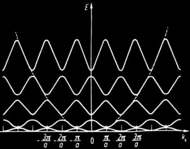
Take a free electron. It would be described by the Schrödinger equation and have a parabollic energy-momentum dispersion. If now you create a periodic lattice in space, the Bloch theorem tells you that you should get a band structure that is periodic in space. The underlying reason is that position and momentum are conjugate variables.

The Floquet states are analogues of Bloch states in the time domain. Since time and energy are conjugate variables, having a time periodicity in the system would result in a periodicity on the energy axis. In condensed matter systems, Floquet states were actually found using ARPES by the group of Nuh Gedik at MIT almost 10 years ago. The way they were observed was by irradiating a topological insulator with a short laser pulse and simultaneously observing the momentum-energy photoemission image. This shows a clear duplication of the band structure in energy: the Floquet states, but with two main drawbacks: a) the Floquet state exists for the time of the impulsion, a few femtoseconds; b) the laser pulse results in considerable heating of the sample.

Let’s now go back to the recent paper in graphene Josephson junctions. These Floquet states are based on Andreev bound states, that can be observed with tunneling spectroscopy as peaks in the dI/dV after the superconducting gap. By irradiating the graphene sample with a microwave excitation, in the same way that one would apply microwaves to observe Shapiro steps, the group of Gil-Ho Lee observed duplicate peaks at energies above and below the Andreev bound states. They characterised these states and provide a definitive proof of the Floquet nature through minute theoretical analysis. Interestingly, the separation between the Floquet states increases with the RF frequency and their number with the power. They also provide a Bessel function analysis (fig 2e) for these, but to me this is not convincing.

The strength of that paper lies in the fact that Floquet states could be found without heating the sample considerably (low frequency allow to use lower electric fields, therefore less heating) and graphene devices present good electron-phonon coupling, allowing continuous cooling in a dilution refrigerator. Additionally, these Floquet states are not volatile. In principle, nothing prevents them from disappearing. The authors claim that the states do not vary for 25h. In principle, this would allow further tuning of the band structure from microwave irradiations.

As I have done previously, I’m writing some words about statistical analysis that I think is useful for undergrads, based on my teaching experience. There is a particularly interesting example posted on arXiv on Tuesday that allows me to illustrate this theory.

Gaussian distribution & Central Limit Theorem

Let’s a set of $n$ independent variables $x_i$ taken at random from a set with mean $\mu$ and variance $\sigma^2$. Now you can calculate the mean $\bar x$ of these $n$ values. The Central Limit Theorem says that the the distribution of $\bar x$ tends to a Gaussian of mean $\mu$ and variance $\sigma^2 / n$. The important feature of the theorem is that whatever the distribution of the $x_i$, a linear combination of a few variables (almost) always approximates to a Gaussian distribution.

What matters here is that acquiring a large number of data with random error leads to a distribution of values that tends to a Gaussian distribution.

In the treatment of errors

A consequence of the Central Limit Theorem is that in most of the situations, repeating an experiment would produce a spread of values whose distribution is a Gaussian. This approximation becomes better if individual errors contributing to the final value are small.

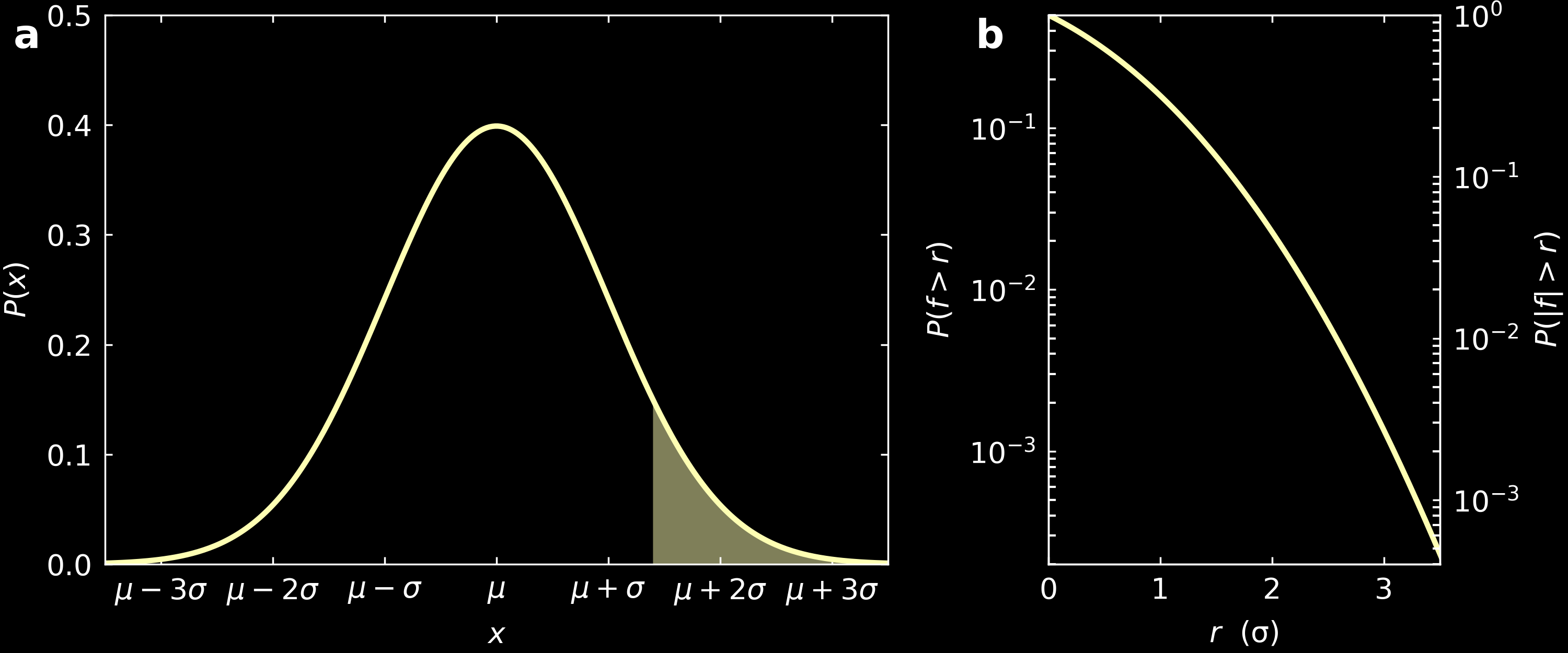
When this is the case, the fractional area in the tail of a Gaussian (filled area in panel (a) of the figure below is always non-zero, for all values $r$ in which it is taken. It is thus meaningless to speak of a maximum possible error of a given experiment as this would be infinite. Although it would be easy to calculate the error on any experiment, that would not distinguish a precise result from an inaccurate one.

Therefore, it is common to quote $\sigma$, the standard deviation of the Gaussian function, as the accuracy for a measurement. As it is not the maximum possible error, results of measurements can fall more than $\sigma$ away form the expected value, without questioning the validity of the assumptions. In fact, $1\sigma$ includes 68% of all the data points, $2\sigma$ includes 95% of all data points, $3\sigma$, 99.7% of all data points, etc.

When we carry out $n$ measurements, the standard deviation $\sigma_m$ of the mean would be calculated as $\sigma_m = \frac{\sigma}{\sqrt{n}}$, that is the standard error in the mean of $n$ observations is $1/\sqrt{n}$ times the standard error in a single observation.

The question of importance now is: when would a particular data point be considered significant? When one data point falls beyond $2\sigma$ away, the probability that it happens is only 5%. When it falls beyond $3\sigma$, the fractional area is only 0.3%, se we would expect a deviation to occur that frequently. As a result, when a data point falls a few sigma away from a model being tested, there is an evidence that the data point is not consistent with the model. Indeed, we should expect a data point to be $3\sigma$ away, about 3 times if the experiment is repeated 1000 times.

Example: LHCb experiment

This preprint from the LHCb collaboration about possible violation of the standard model, that had a good press coverage.

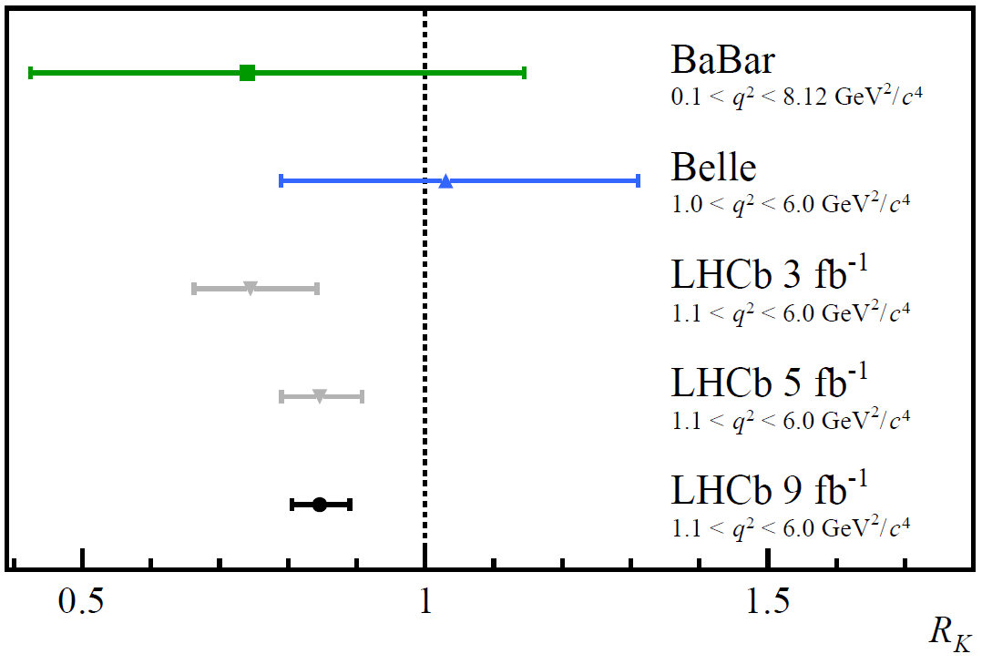
They measure the decay of beauty quarks (B-mesons) into muons and electrons, probed through the value $R_K$ that is the ratio between these two decays and find $R_K$ = 0.846 $\pm$ 0.044 (that includes a statistical error evaluated at +0.042/-0.039 and a systematic error evaluated at +0.013/-0.012). The standard model would predict a value of 1.00$\pm$0.01. The question is: to what extent are these numbers in agreement?

To answer this, let’s look at panel b in the above figure. This shows the fractional area under the gaussian curve ($|f|>r$ with $f = \frac{x-\mu}{\sigma}$), that is the area of the tail highlighted in panel a. In the LHCb example, $\mu$ = 1, $\sigma$ = 0.044 and $x$ = 0.846. With our formula, this gives $f=3.5$, for which the corresponding probability read on the graph is 0.046%. In reality, they evaluate this more precisely than my rough analysis and get $f=3.1$ with a corresponding probability of 0.1%.

As a result, if 1000 experiments are performed, all of which with the same precision and if the theory is correct and if the experiment is bias-free, then we expect about 1 of them to differ from this value at least as much as this experiment does. The scientists of the LHCb collaboration expect to repeat update the experimental setup to go as far as $5\sigma$, that would give a probability of 6·10⁻⁵%. What will matter in this case is whether they regard the theory (and the experiment) as satisfactory or not, but they will have numbers to base that judgement on.

What this example means, is that if the Standard Model is valid (the Null hypothesis), there is 1 in 10,000 chance the LHCb data is at least as extreme as what they observed. In this field, this is still not enough to claim they found something outside of the Standard Model.

A week ago we published a paper in Nature physics showing the formation of van Hove singularities in twisted monolayer-bilayer graphene systems that can be tuned with the application of an electric field or by changing the twist angle. Notably, we show that these can cause strong correlations effects under various conditions. This is an interesting system, reproducing strongly correlated states seen in magic-angle graphene, but for some reason much easier to process.

Role of symmetry

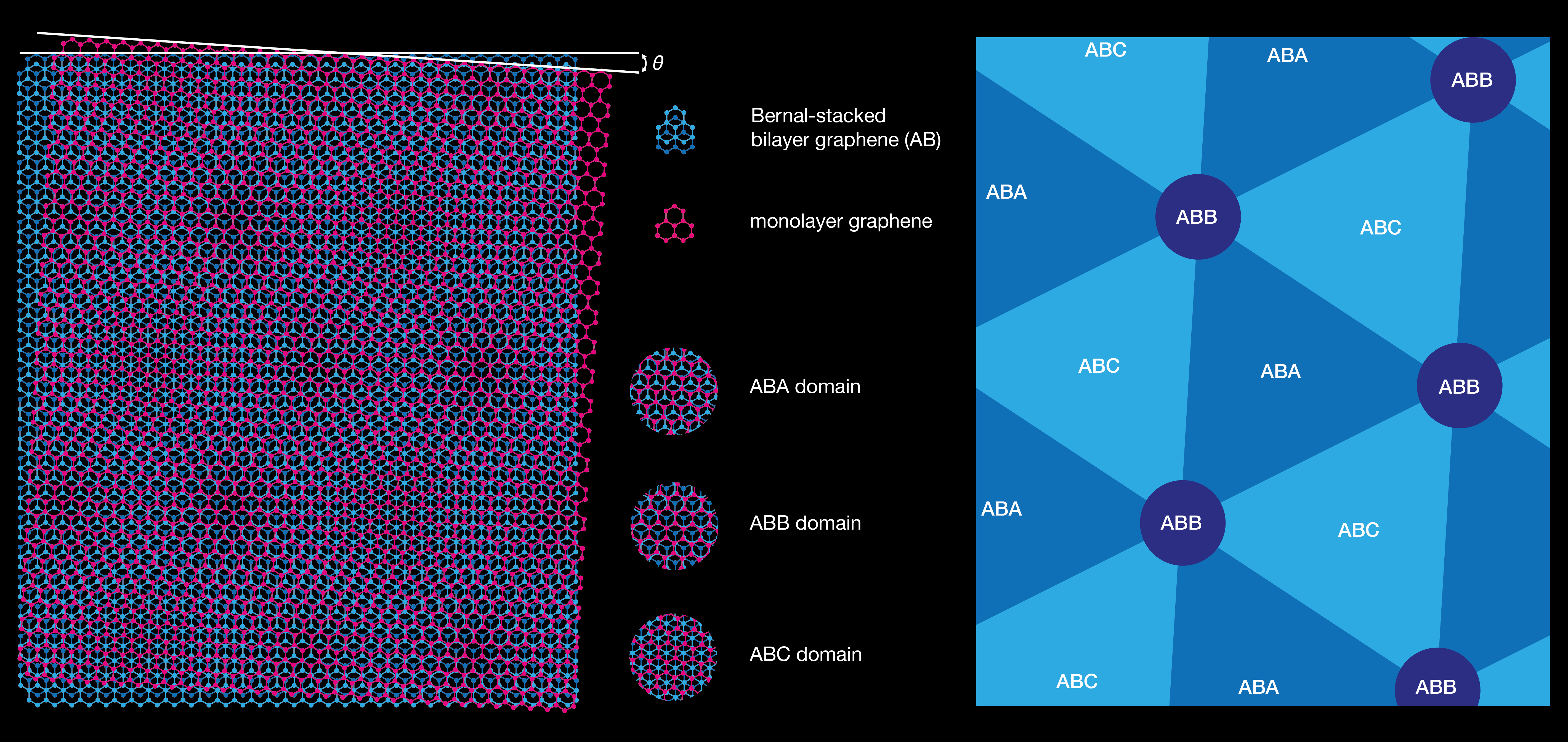
Twisted van der Waals heterostructures usually offer different tuning parameters to create exotic state. In the case of twisted monolayer-bilayer graphene, there are more tuning knobs, compared to twisted bilayer graphene, because the band structure of multilayer graphene (here, bi-layer) is more tuneable than the one of the monolayer. Different stacking orders can exist for trilayer graphene: Bernal (ABA) or rhombohedral (ABC). The former presents a mirror symmetry and is semi-metallic, whereas the latter presents an inversion symmetry and is semi-conducting, with a gap that can be varied with the displacement field.

In twisted monolayer-bilayer graphene, the symmetry is even more reduced with the twist induced between the bilayer and monolayer graphene, that results in ABA-, ABB- and ABC-domains (cf schematic below).

The phase diagram can be tuned via field-effect

In all the studies, twisted monolayer-bilayer graphene (tMBG) devices comprise a top- and back-gate, that allow to control the doping ($n$) or to apply a perpendicular electric field in the material ($D$).

Particularly, Chen et al have shown that a variety of correlated metallic, insulating and topological magnetic state appear, owing to the low symmetry. Particularly, the application of a displacement field endows this system with either the phase diagram of twisted bilayer graphene (at positive displacements) or twisted double bilayer graphene (at negative displacements).

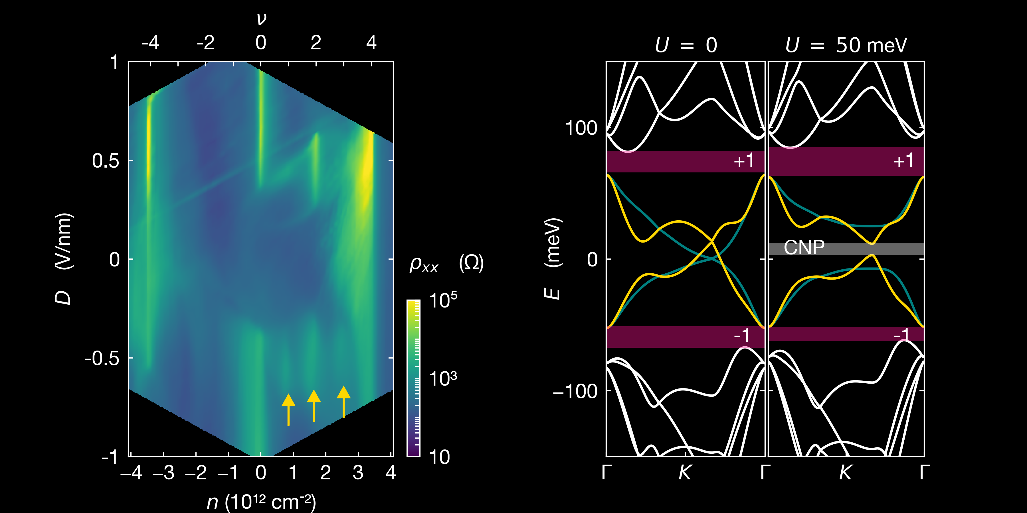
We (Xu et al) have studied tMBG devices with a twist between 1.2° and 1.6° and studied the correlated states that appear asymetrically with the external electric field applied between the layer, and are highly tuneable by varying the twist angle. As shown on the following figure, two resistive peaks emerge at full filling $\nu = \pm 4$, and a gap opens at charge neutrality point (CNP) with increased $D$. The single particle model cannot explain the resistive and metallic states at half and quarter fillings. We have shown that the resistivity is asymmetric for electrons and holes in these states.

Correlated states at quarter filling

Polshyn et al have observed the correlated states corresponding to filling of 1 and 3 electrons per unit cell. In these states, they observe a quantised anomalous hall effect, with a transverse resistance close to $h/2e^2$. This could indicate a spontaneous polarisation of the system into a single-valley projected band. In the state with 3 electrons per unit cell, they show, as well, that the sign of the quantum anomalous hall effect can be reversed via field-effect control of the chemical potential. This is a major breakthrough.

Chen et al observe these correlated states undergoing an orbitally-driven insulating transition above a critical perpendicular magnetic field, for electric fields applied from the monolayer to the bilayer ($D>0$). Particularly, at $\nu = 1$ (one electron per moiré unit cell), they probe the emergence of an electrically tuneable ferromagnetism, in the conduction band, that is accompanied by an anomalous Hall effect.

More recently, He et al reported that orbital magnetism is abundant within the correlated phase diagram, leading to anomalous Hall states within the correlated metallic states around odd integer fillings of the flat conduction band. They also observe correlated Chern insulator that are stabilised within a magnetic field. Importantly, they show that this behaviour at zero electric field is inconsistent with simple spin and valley polarisation and propose an intervalley coherent state with an order parameter, breaking time-reversal symmetry.

All these study show that both electric and magnetic field can tune competition between correlated and topological phase, owing to the rich interplay between competing correlated states in twisted monolayer-bilayer graphene systems. So far, most of the recent study focused in the conduction band at $D>0$, where the system has a phase diagram comparable to twisted double bilayer graphene.

References:

• H. Polshyn et al 2020, Electrical switching of magnetic order in an orbital Chern insulator, Nature;
• S. Chen et al 2020, Electrically tunable correlated and topological states in twisted monolayer-bilayer graphene, Nature Physics;
• S. Xu, et al 2021, Tunable van Hove singularities and correlated states in twisted monolayer-bilayer graphene, Nature Physics;
• M. He et al 2021, Competing correlated states and abundant orbital magnetism in twisted monolayer-bilayer graphene.

This semester I’ve been teaching foundation year students in experimental physics. The goal for them is to find a laser’s wavelength through diffraction experiments. Because of the covid-19 pandemic, restrictions imposed by the University don’t allow the students in labs, so I have to carry out the experiment, filmed with different cameras and broadcasted to the students at home. The far-from-ideal situation led to poor accuracy in the measurement readings, hence a substantial errors on each of their measure. I’ve noticed that this was a source of issues, as many sent me e-mails or came to the drop-in session, to understand why their measurements did not match the expected value. This actually leads to some interesting discussions about experimental errors. I’d like to share some of this.

Why we estimate errors

The foundation year students come to the class with the (justified) feeling that the job is done once they obtain a numerical value for the quantity we ask them to measure or calculate. This is different at university, as we are also concerned with the accuracy of the measurement. The accuracy is expressed with an experimental error on the measurement. As we, scientists, are interested in measurements for the sake of comparing them with different experiments, theories, or use them to predict new behaviours, the value of the error becomes crucial to the interpretation of the result. Let me develop this.

In my lab, the students are asked to find the wavelength of a laser. We give them the laser specification (including the wavelength), and most of the time, they get something different from the specification. The laser’s wavelength is supposed to be 532nm (green light beam). When they measure 528nm, how can we get an evidence for a discrepancy? Can we conclude directly that the laser’s specification is inacurate? There could be 3 possibilities:

1. if the experimental error is $\pm 5$nm then this result looks satisfactory, and in agreement with the expected value: 528±5 is consistent with 532
2. if the experimental error is $\pm 0.5$nm then the measurement loos inconsistent with the expected value. We should worry that either the experimental result or the error estimate is wrong. Another possibility is that the specification for the laser is different from its real value: 528.0±0.5 is inconsistent with 532
3. if the experimental error is $\pm50$nm (that may happen if we take only one measurement) then the result is consistent with the expectation. However, the accuracy is so low that we will be unable to detect significant differences. The range of confidence of this result would be 478 to 578nm, that is from blue to yellow: a rough estimation would do better.

For a given measurement the interpretation (our measurement is accurate, the laser specifications are inaccurate or we should find how to do a more precise experiment) depends only on the uncertainty of this measurement. If we don’t know it, we are completely unable to judge the significance of the result.

Definition of the experimental error

The measurement error (or observational error), $\delta x$, is the difference between the measured value $x$ for a determined quantity, and its true value $X$. Note that in this context, an error is not a mistake. We can write $X = x + \delta x$

This is a notion that is essential in experimental physics. There are two kinds of errors: random error and systematic error:

Random error

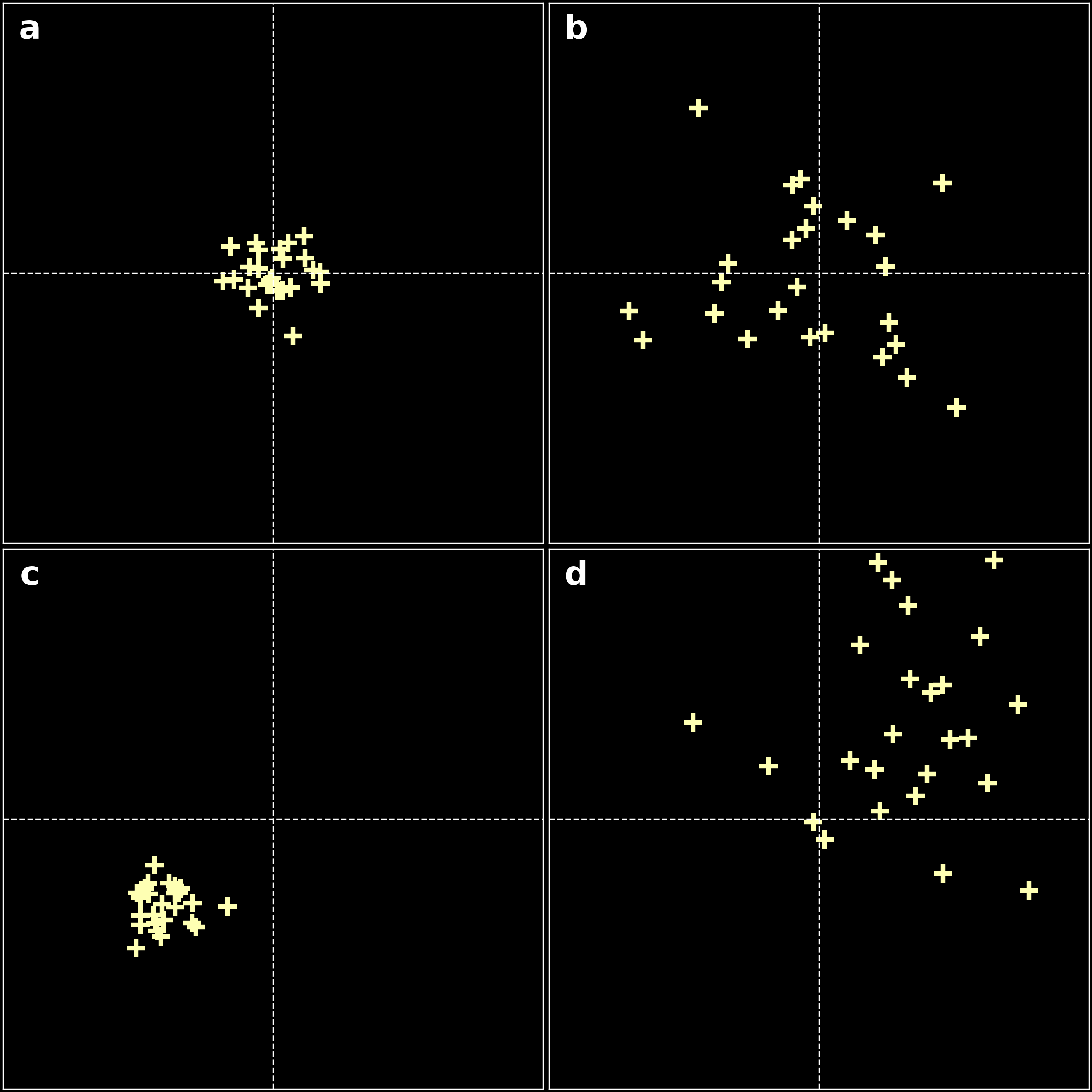
When we measure a physical quantity in the lab, we find that repeating the experiment results in slightly different measures. In my lab that can be due to inaccuracy of reading distances from a ruler that is filmed, for example. It comes from the inability of any measuring device (and to certain extent, to the scientist) to give infinitely accurate measures. This phenomenon is called random error and will be detected through a statistical analysis. Usually, the result of the measure is characterised by a probability distribution, centred around the true value for pure random error (see panel b in the figure below).

Systematic errors

Systematic errors are errors that do not vary with repeated measurements. They result in a measurement that is simply wrong or biased. In my lab, I place a diffraction grating on a ruler. If this grating is not exactly aligned at the center of the reading, statistical studies will not detect the error. Panel c in the figure below shows an example of a systematic error. Generally, systematic errors can have various origins:

• calibration error: A famous example is the experience of Millikan. He found a wrong value of the electron charge as he considered a wrong value for the air viscosity.
• omitted parameter: Suppose that we measure a spin echo. The spin relaxation time would depend on the temperature. Carrying out the measurement in Portugal or Finland without accounting for the temperature would give two different results.
• flawed procedure: Suppose we are measuring a resistance. If the impedance of the voltmeter is not large enough, the approximation of a constant current through the resistor will no longer be valid. Systematic errors are hard to detect, but once they are known, they can be accounted for easily.

As shown on the figure above when making a series of repeated measurements, the effect of random errors will produce a spread of measures scattered around the true value. Systematic errors on the contrary would cause the measurement to be offset from the correct value, even when individual measurements are consistent with one another.

Difference between error and uncertainty

I have found that both uncertainty and errors are mistaken, some students talking about calculating errors instead of uncertainty. This is sometimes true for established scientists.

The uncertainty $\Delta x$ estimates the importance of the random error. Without a systematic error, the uncertainty defines an interval around the measured value, that includes the true value with a determined confidence level (usually 2/3) We can estimate this two ways:

statistically (type A)

In this method we characterise the probability distribution of the $x$ values. With a good evaluation of the mean and the standard deviation of the distribution. This is done through statistical analysis over an ensemble of measures of $x$. Without systematic error, the mean value is the best estimate of the true value $X$, while the uncertainty $\Delta x$ is directly linked to the standard deviation of the distribution, and defines an interval in which the true value $X$ can be found with a known confidence level.

other means (type B)

When we have no time or resources to make additional measurements, we estimate $\Delta x$ from the specifications of the measurement instruments. For example, in the experiment I carry out in my lab, we can estimate the uncertainty in the number of lines per millimeter in the diffraction grating to be around 5%. For 300lines per millimeter, that would result in an uncertainty of $300\pm15$l/mm. When reading the position of that diffraction grating on the ruler, we can estimate the uncertainty on the reading of about half to one graduation. When reading numeric values, we typically find a precision $\Delta$ on the measure that is $\pm 2$ times the last digit and $\pm 0.1\%$ of the measured value. This, of course, depends on the quality of the instrument and calibration, and can be found in the specifications of the instrument. Calibration error is mostly accounted for in the 0.1% part of the value we read. Noise and random errors are typically found in the last digit. When we evaluate the uncertainty over a measure with a type B method, we usually divide the precision $\Delta$ by $\sqrt{3}$ (that supposes a uniform probability distribution of width $2\Delta$).

Estimating the uncertainty with a type A method

Each time we record a measure in which the source of error is purely random, we are likely to record a different value to the previous measurement. In that case, a set of repeated measurements of $x$ would give an estimate of $\Delta x$. It is likely that the dispersion of the measurements is larger than the individual error on each measurements. In that case, the standard dispersion will be used as the uncertainty: \[ \Delta x \approx \sqrt{\frac{N}{N-1}} s \] With $s$ the standard deviation of a set of $N$ measurements.

The mean value will be given by: \[ \left< x \right> = \frac{1}{N} \sum_{i=1}^N x_i \] where $x_i$ are the individual measurements in the set. Since the mean value of the set is statistically more likely to be close to the true value than any one of the individual measurement chosen at random, the uncertainty of the mean value, $\sigma_m$ is smaller than the uncertainty $\delta x$ of any one of the measurement. We can prove that $\sigma_m = \frac{\delta x}{\sqrt{N}}$.

What it means in undergrad labs

In the lab, the uncertainty is an essential value to judge the accuracy of a measurement, that makes us able to judge of the quality of a measure. There are good practices to mitigate the influence of errors and reduce the uncertainty of a measurement. The first is to analyse statistically, whenever it is possible, the value, and consider only the mean values, with the associated uncertainty. Second, I would also recommend to record everything that could be relevant to the problem on a neat notebook. It becomes all the more important in the remote lab to write down results manually, with an estimation of their uncertainty, as soon as they are collected: you cannot mitigate errors if you don’t record them in the first place.

references

• Data Analysis for Physical Science Students, L. Lyons, Cambridge University Press 1991
• Practical Physics, G. L. Squires, Cambridge University Press 2001

The past semester, I have been teaching in the physics third year lab. One of the experiments consists in emasuring the electrical resistivity of a graphene layer with a lock-in amplifier.

Before this lab, to measure a resistence, students are used to use a d.c. potentiometer to measure an electrical resistance, so I could notice some qualm about the new technique. The d.c. potentiometer is an easy system for such applications, but prone to measurement errors because of thermoelectric and drift effects that can be hard to eliminate, as well as issues when the measured signal falls below the error voltage of the instrument. For this reason, methods involvig the use of an a.c. current allow for more precise electrical measurements. In fact, if one applies an a.c. current and measure the differential output voltage, between successive maxima and minima (or, more conveniently, the root mean square of this value, $V_{rms}$) and interval this over a number of modulation cicles, one can get an improved estimate of the voltage difference, that eliminates the thermal drifts and low-frequency noise.

I think this method is of particular importance in modern mesoscopic physics, and justifies a few words on this blog.

The lock-in method.

The basic experimental arrangement in lock-in detection in a four-probe configuration consists in the following: a sine-wave current is generated at a frequency $f_0$ and constant amplitude and passed through a pair of contacts (A and B for example) of the measured device, and a voltage drop across another pair of contacts (C and D) is measured with the lock-in amplifier. This acts as a highly-tuned demodulator, and gives a d.c. output that is proportional to the amplitude of the a.c. voltage $V$ between C and D. The essential feature of the lock-in amplifier is that it works at the reference signal of frequency $f_0$, that has the same frequency as the sample. This methods allows to measure a current and a voltage with a precision of about 1 part in 10⁴.

Importance of phase-sensitive detection

As I just wrote, a lock-in is a phase-sensitive detector, measuring the difference voltage of interest, using a synchronous reference voltage. Detection with respect to a synchronous reference allows to use long averaging time to be able to improve the detection below background noise level. This is important in comparison to the use of amplitude demodulation with non-linear devices (like enveloppe detectors), that would make no difference between the signal and noise components. The phase-sensitive detector would measure only the frequency of interest $f_0$. Lock-in amplifiers are usually able to measure both the amplitude of the voltage, and the phase difference.

Noise reduction.

In a typical measurement, the resistance of metallic samples can vary from 10^-3Ω at room temperature, to 10^-6Ω at low temperatures. In the Kelvin-range, a few millivolts can heat a device substantially and counterbalance all the efforts made to reach low-temperatures. Under such conditions, the maximum range that can decently be used is about 10µV, so the measured voltage drop would be in the order of the nanovolt. In a typical experiment, leads from room temperature to liquid-helium temperatures would carry a thermoelectric voltage (noise) in the order of the µV to the mV. It is thus necessary to be able to measure below the noise level. Synchronous detection allows to single out the component of the signal at a specific reference frequency and noise, therefore reducing the measured noise.

There are three main types of noise: Johnson (or thermal) noise, shot noise and 1/f noise.

Johnson noise

Every resistive system would generate a noise voltage at its therminal, that is due to the thermal fluctuations of the electron density. We can characterise the noise as: \[ V_{JN} = \sqrt{4k_B T R \Delta f} \] where $k_B$ is Boltzmann’s constant, $T$ the temperature of the sample of interest, $R$ its resistance and $\Delta f$ the bandwith of the measurement. This means that the amount of noise that is captured by the lock-in is determined directly by the bandwidth of the input signal. State of the art lock-ins would have a bandwidth frequency around 500kHz, that means an effective noise at 300K, at the amplifier input that is $V_{JN} \approx 40\sqrt{R}$nV. Here, high input bandwidth allow to reduce Johnson noise.

Shot noise

Shot noise comes from the discrete nature of the charge carriers. As there is always non-uniformities in the electron flow generating current noise, the shot noise would be given by: \[ I_{SN} = \sqrt{2qI_{a.c.}\Delta f} \] where $q$ is the electron charge, $I_{a.c.}$ the current and $\Delta f$ the bandwidth. With a lock-in, this is minimal (that is $I_{SN} \approx 400\sqrt{I_{a.c.}}$10^-9).

1/f noise (or Flicker noise)

Flicker noise results fluctuations in resistance due to a current flowing through the resistor. It can be between 10nV and 1µV per volt applied across a resistor, with a 1/f spectrum. As a result, measurements at low frequencies are noisier.

References

• Betts, J.A, Signal processing, modulation and noise, London 1970
• Meade, ML, Lock-in amplifiers: principles and applications, London 2013
• Principles of lock-in detection and the state of the art, Zurich Instruments white paper, 2016.