 0000-0002-6484-2157
As I have done previously, I’m writing some words about statistical analysis that I think is useful for undergrads, based on my teaching experience. There is a particularly interesting example posted on arXiv on Tuesday that allows me to illustrate this theory.
Gaussian distribution & Central Limit Theorem
Let’s a set of $n$ independent variables $x_i$ taken at random from a set with mean $\mu$ and variance $\sigma^2$. Now you can calculate the mean $\bar x$ of these $n$ values. The Central Limit Theorem says that the the distribution of $\bar x$ tends to a Gaussian of mean $\mu$ and variance $\sigma^2 / n$. The important feature of the theorem is that whatever the distribution of the $x_i$, a linear combination of a few variables (almost) always approximates to a Gaussian distribution.
What matters here is that acquiring a large number of data with random error leads to a distribution of values that tends to a Gaussian distribution.
In the treatment of errors
A consequence of the Central Limit Theorem is that in most of the situations, repeating an experiment would produce a spread of values whose distribution is a Gaussian. This approximation becomes better if individual errors contributing to the final value are small.
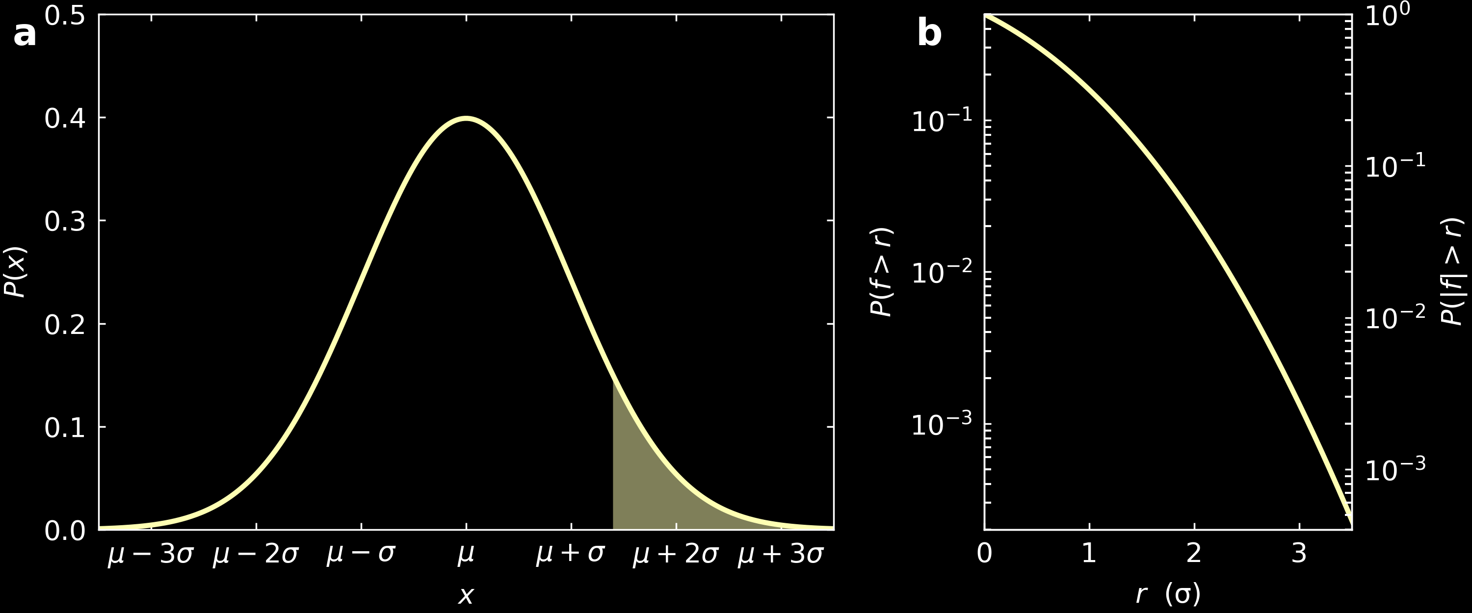
When this is the case, the fractional area in the tail of a Gaussian (filled area in panel (a) of the figure below is always non-zero, for all values $r$ in which it is taken. It is thus meaningless to speak of a maximum possible error of a given experiment as this would be infinite. Although it would be easy to calculate the error on any experiment, that would not distinguish a precise result from an inaccurate one.
Therefore, it is common to quote $\sigma$, the standard deviation of the Gaussian function, as the accuracy for a measurement. As it is not the maximum possible error, results of measurements can fall more than $\sigma$ away form the expected value, without questioning the validity of the assumptions. In fact, $1\sigma$ includes 68% of all the data points, $2\sigma$ includes 95% of all data points, $3\sigma$, 99.7% of all data points, etc.
When we carry out $n$ measurements, the standard deviation $\sigma_m$ of the mean would be calculated as $\sigma_m = \frac{\sigma}{\sqrt{n}}$, that is the standard error in the mean of $n$ observations is $1/\sqrt{n}$ times the standard error in a single observation.
The question of importance now is: when would a particular data point be considered significant? When one data point falls beyond $2\sigma$ away, the probability that it happens is only 5%. When it falls beyond $3\sigma$, the fractional area is only 0.3%, se we would expect a deviation to occur that frequently. As a result, when a data point falls a few sigma away from a model being tested, there is an evidence that the data point is not consistent with the model. Indeed, we should expect a data point to be $3\sigma$ away, about 3 times if the experiment is repeated 1000 times.
Example: LHCb experiment
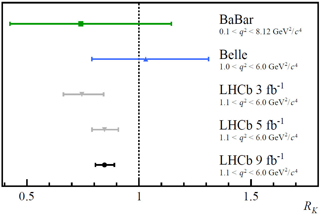
This preprint from the LHCb collaboration about possible violation of the standard model, that had a good press coverage.
They measure the decay of beauty quarks (B-mesons) into muons and electrons, probed through the value $R_K$ that is the ratio between these two decays and find $R_K$ = 0.846 $\pm$ 0.044 (that includes a statistical error evaluated at +0.042/-0.039 and a systematic error evaluated at +0.013/-0.012). The standard model would predict a value of 1.00$\pm$0.01. The question is: to what extent are these numbers in agreement?
To answer this, let’s look at panel b in the above figure. This shows the fractional area under the gaussian curve ($|f|>r$ with $f = \frac{x-\mu}{\sigma}$), that is the area of the tail highlighted in panel a. In the LHCb example, $\mu$ = 1, $\sigma$ = 0.044 and $x$ = 0.846. With our formula, this gives $f=3.5$, for which the corresponding probability read on the graph is 0.046%. In reality, they evaluate this more precisely than my rough analysis and get $f=3.1$ with a corresponding probability of 0.1%.
As a result, if 1000 experiments are performed, all of which with the same precision and if the theory is correct and if the experiment is bias-free, then we expect about 1 of them to differ from this value at least as much as this experiment does. The scientists of the LHCb collaboration expect to repeat update the experimental setup to go as far as $5\sigma$, that would give a probability of 6·10⁻⁵%. What will matter in this case is whether they regard the theory (and the experiment) as satisfactory or not, but they will have numbers to base that judgement on.
What this example means, is that if the Standard Model is valid (the Null hypothesis), there is 1 in 10,000 chance the LHCb data is at least as extreme as what they observed. In this field, this is still not enough to claim they found something outside of the Standard Model.