This semester I’ve been teaching foundation year students in experimental physics. The goal for them is to find a laser’s wavelength through diffraction experiments. Because of the covid-19 pandemic, restrictions imposed by the University don’t allow the students in labs, so I have to carry out the experiment, filmed with different cameras and broadcasted to the students at home. The far-from-ideal situation led to poor accuracy in the measurement readings, hence a substantial errors on each of their measure. I’ve noticed that this was a source of issues, as many sent me e-mails or came to the drop-in session, to understand why their measurements did not match the expected value. This actually leads to some interesting discussions about experimental errors. I’d like to share some of this.

Why we estimate errors

The foundation year students come to the class with the (justified) feeling that the job is done once they obtain a numerical value for the quantity we ask them to measure or calculate. This is different at university, as we are also concerned with the accuracy of the measurement. The accuracy is expressed with an experimental error on the measurement. As we, scientists, are interested in measurements for the sake of comparing them with different experiments, theories, or use them to predict new behaviours, the value of the error becomes crucial to the interpretation of the result. Let me develop this.

In my lab, the students are asked to find the wavelength of a laser. We give them the laser specification (including the wavelength), and most of the time, they get something different from the specification. The laser’s wavelength is supposed to be 532nm (green light beam). When they measure 528nm, how can we get an evidence for a discrepancy? Can we conclude directly that the laser’s specification is inacurate? There could be 3 possibilities:

1. if the experimental error is $\pm 5$nm then this result looks satisfactory, and in agreement with the expected value: 528±5 is consistent with 532
2. if the experimental error is $\pm 0.5$nm then the measurement loos inconsistent with the expected value. We should worry that either the experimental result or the error estimate is wrong. Another possibility is that the specification for the laser is different from its real value: 528.0±0.5 is inconsistent with 532
3. if the experimental error is $\pm50$nm (that may happen if we take only one measurement) then the result is consistent with the expectation. However, the accuracy is so low that we will be unable to detect significant differences. The range of confidence of this result would be 478 to 578nm, that is from blue to yellow: a rough estimation would do better.

For a given measurement the interpretation (our measurement is accurate, the laser specifications are inaccurate or we should find how to do a more precise experiment) depends only on the uncertainty of this measurement. If we don’t know it, we are completely unable to judge the significance of the result.

Definition of the experimental error

The measurement error (or observational error), $\delta x$, is the difference between the measured value $x$ for a determined quantity, and its true value $X$. Note that in this context, an error is not a mistake. We can write $X = x + \delta x$

This is a notion that is essential in experimental physics. There are two kinds of errors: random error and systematic error:

Random error

When we measure a physical quantity in the lab, we find that repeating the experiment results in slightly different measures. In my lab that can be due to inaccuracy of reading distances from a ruler that is filmed, for example. It comes from the inability of any measuring device (and to certain extent, to the scientist) to give infinitely accurate measures. This phenomenon is called random error and will be detected through a statistical analysis. Usually, the result of the measure is characterised by a probability distribution, centred around the true value for pure random error (see panel b in the figure below).

Systematic errors

Systematic errors are errors that do not vary with repeated measurements. They result in a measurement that is simply wrong or biased. In my lab, I place a diffraction grating on a ruler. If this grating is not exactly aligned at the center of the reading, statistical studies will not detect the error. Panel c in the figure below shows an example of a systematic error. Generally, systematic errors can have various origins:

• calibration error: A famous example is the experience of Millikan. He found a wrong value of the electron charge as he considered a wrong value for the air viscosity.
• omitted parameter: Suppose that we measure a spin echo. The spin relaxation time would depend on the temperature. Carrying out the measurement in Portugal or Finland without accounting for the temperature would give two different results.
• flawed procedure: Suppose we are measuring a resistance. If the impedance of the voltmeter is not large enough, the approximation of a constant current through the resistor will no longer be valid. Systematic errors are hard to detect, but once they are known, they can be accounted for easily.

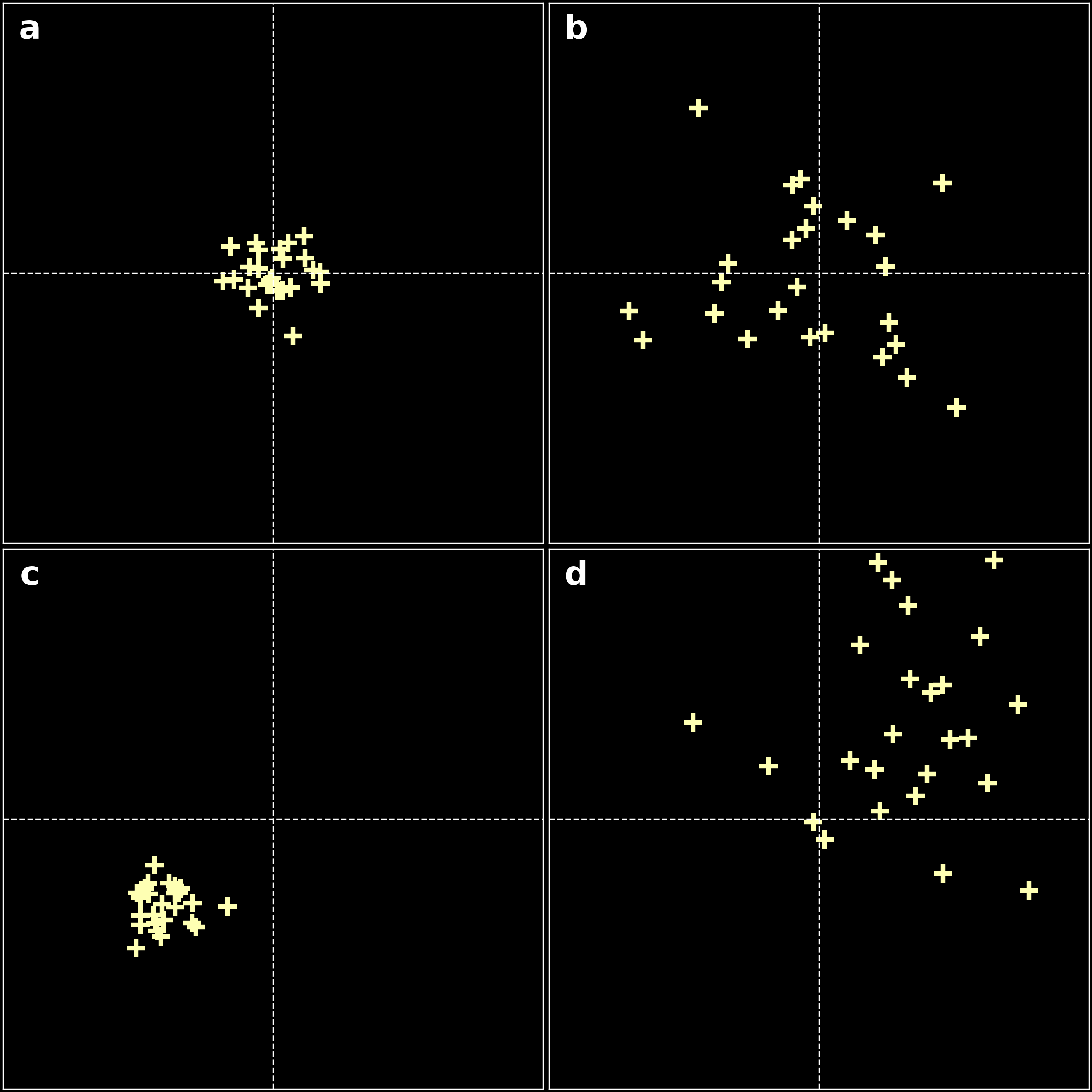
As shown on the figure above when making a series of repeated measurements, the effect of random errors will produce a spread of measures scattered around the true value. Systematic errors on the contrary would cause the measurement to be offset from the correct value, even when individual measurements are consistent with one another.

Difference between error and uncertainty

I have found that both uncertainty and errors are mistaken, some students talking about calculating errors instead of uncertainty. This is sometimes true for established scientists.

The uncertainty $\Delta x$ estimates the importance of the random error. Without a systematic error, the uncertainty defines an interval around the measured value, that includes the true value with a determined confidence level (usually 2/3) We can estimate this two ways:

statistically (type A)

In this method we characterise the probability distribution of the $x$ values. With a good evaluation of the mean and the standard deviation of the distribution. This is done through statistical analysis over an ensemble of measures of $x$. Without systematic error, the mean value is the best estimate of the true value $X$, while the uncertainty $\Delta x$ is directly linked to the standard deviation of the distribution, and defines an interval in which the true value $X$ can be found with a known confidence level.

other means (type B)

When we have no time or resources to make additional measurements, we estimate $\Delta x$ from the specifications of the measurement instruments. For example, in the experiment I carry out in my lab, we can estimate the uncertainty in the number of lines per millimeter in the diffraction grating to be around 5%. For 300lines per millimeter, that would result in an uncertainty of $300\pm15$l/mm. When reading the position of that diffraction grating on the ruler, we can estimate the uncertainty on the reading of about half to one graduation. When reading numeric values, we typically find a precision $\Delta$ on the measure that is $\pm 2$ times the last digit and $\pm 0.1\%$ of the measured value. This, of course, depends on the quality of the instrument and calibration, and can be found in the specifications of the instrument. Calibration error is mostly accounted for in the 0.1% part of the value we read. Noise and random errors are typically found in the last digit. When we evaluate the uncertainty over a measure with a type B method, we usually divide the precision $\Delta$ by $\sqrt{3}$ (that supposes a uniform probability distribution of width $2\Delta$).

Estimating the uncertainty with a type A method

Each time we record a measure in which the source of error is purely random, we are likely to record a different value to the previous measurement. In that case, a set of repeated measurements of $x$ would give an estimate of $\Delta x$. It is likely that the dispersion of the measurements is larger than the individual error on each measurements. In that case, the standard dispersion will be used as the uncertainty: \[ \Delta x \approx \sqrt{\frac{N}{N-1}} s \] With $s$ the standard deviation of a set of $N$ measurements.

The mean value will be given by: \[ \left< x \right> = \frac{1}{N} \sum_{i=1}^N x_i \] where $x_i$ are the individual measurements in the set. Since the mean value of the set is statistically more likely to be close to the true value than any one of the individual measurement chosen at random, the uncertainty of the mean value, $\sigma_m$ is smaller than the uncertainty $\delta x$ of any one of the measurement. We can prove that $\sigma_m = \frac{\delta x}{\sqrt{N}}$.

What it means in undergrad labs

In the lab, the uncertainty is an essential value to judge the accuracy of a measurement, that makes us able to judge of the quality of a measure. There are good practices to mitigate the influence of errors and reduce the uncertainty of a measurement. The first is to analyse statistically, whenever it is possible, the value, and consider only the mean values, with the associated uncertainty. Second, I would also recommend to record everything that could be relevant to the problem on a neat notebook. It becomes all the more important in the remote lab to write down results manually, with an estimation of their uncertainty, as soon as they are collected: you cannot mitigate errors if you don’t record them in the first place.

references

• Data Analysis for Physical Science Students, L. Lyons, Cambridge University Press 1991
• Practical Physics, G. L. Squires, Cambridge University Press 2001